
The Poisson Distribution
- Marek Vavrovic
- May 28, 2020
- 5 min read
Updated: May 30, 2020
The Poisson distribution is a mathematical concept for converting the overall average into probabilities for different results. A Poisson experiment is a statistical experiment that has the following properties:
The experiment results in outcomes that can be classified as successes or failures.
The average number of successes (μ) that occurs in a specified region is known.
The probability that a success will occur is proportional to the size of the region.
The probability that a success will occur in an extremely small region is virtually zero.
The Poisson distribution and the Binomial distribution have some similarities, but also several differences. The binomial distribution describes a distribution of two possible outcomes designated as successes and failures from a given number of trials. Only 2 possible outcomes. The Poisson distribution focuses only on the number of discrete occurrences over some interval. Can be unlimited number of possible outcomes.
The Poisson distribution arises in two ways:
1. Events distributed independently of one another in time:
X = the number of events occurring in a fixed time interval has a Poisson distribution.

2. As an approximation to the binomial when p is small and n is large. When examining the number of defectives in a large batch= [n] where [p]=the defective rate, is usually small.
EXAMPLE
The manufacturer of the disk drives in one of the well-known brands of microcomputers expects 2% of the disk drives to malfunction during the microccomputer’s warranty period.
Calculate the probability that in a sample of 100 disk drives, that not more than 3 will malfunction.
Poisson as an approximation to the binomial when n is large p is small:
• mean of binomial = np
• mean of Poisson = λ
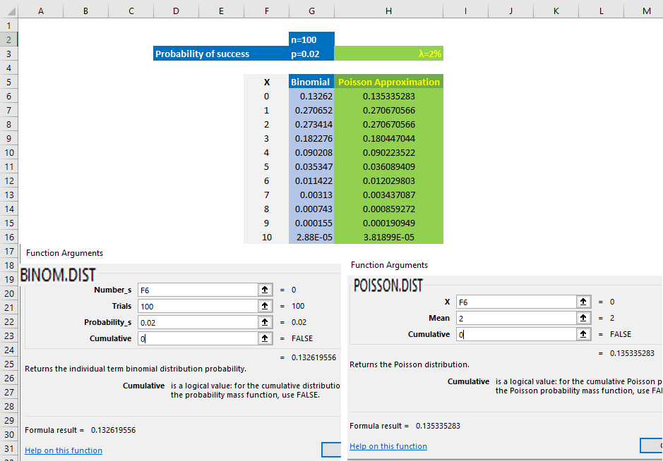
Have a look on the charts....

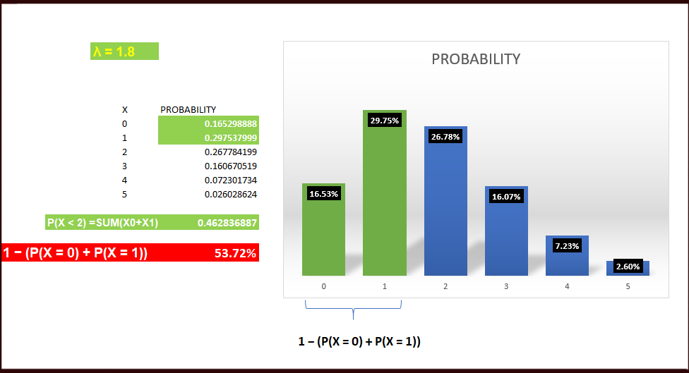
Example: Hospital births.
Births in a hospital occur randomly at an average rate of 1.8 births per hour. What is the probability of observing 4 births in a given hour at the hospital?
(i) Events occur randomly
(ii) Mean rate λ = 1.8

What is the probability of observing more than or equal to 2 births in a given hour at the hospital?
We want P(X ≥ 2) = P(X = 2) + P(X = 3) + . . . i.e. an infinite number of probabilities to calculate.
But:
P(X ≥ 2) = 1 − P(X < 2)
= 1 − (P(X = 0) + P(X = 1))
= 53.72%
Example: Disease incidence.
Suppose there is a disease, whose average incidence is 2 per million people. What is the probability that a city of 1 million people has at least twice the average incidence?
Twice the average incidence would be 4 cases.
We can reasonably suppose the random variable
X=number of cases in 1 million people has
Poisson distribution with parameter 2.
Then
P(X ≥ 4) = 1 − P(X ≤ 3)=14.29%

We observe that the Poisson distributions
1. are unimodal
2. exhibit positive skew (that decreases as λ increases)
3. are centred roughly on λ
4. have variance (spread) that increases as λ increases.
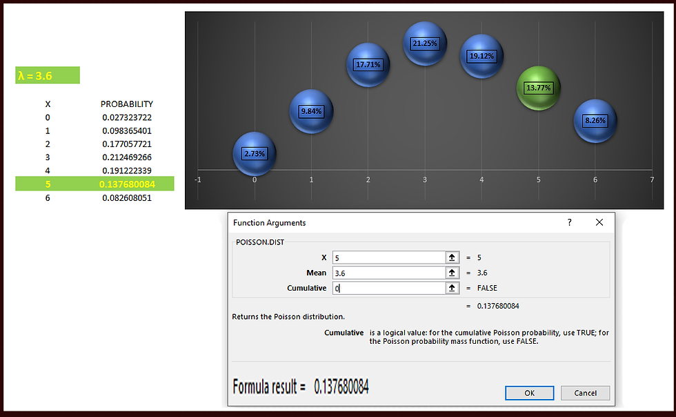
Example: Hospital. [Changing the size of the interval]
Suppose we know that births in a hospital occur randomly at an average rate of 1.8 births per hour. What is the probability that we observe 5 births in a given 2 hour interval?
If births occur randomly at a rate of 1.8 births per 1 hour interval,
then births occur randomly at a rate of 3.6 births per 2 hour interval.
λ =3.6
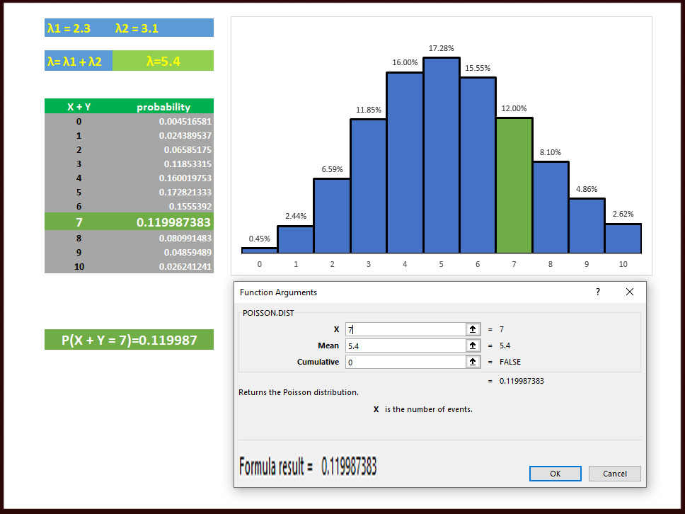
Example: Hospital. [Sum of two Poisson variables]
Now suppose we know that:
in hospital A births occur randomly at an average rate of 2.3 births per hour.
in hospital B births occur randomly at an average rate of 3.1 births per hour.
What is the probability that we observe 7 births in total from the two hospitals in a given 1 hour period?
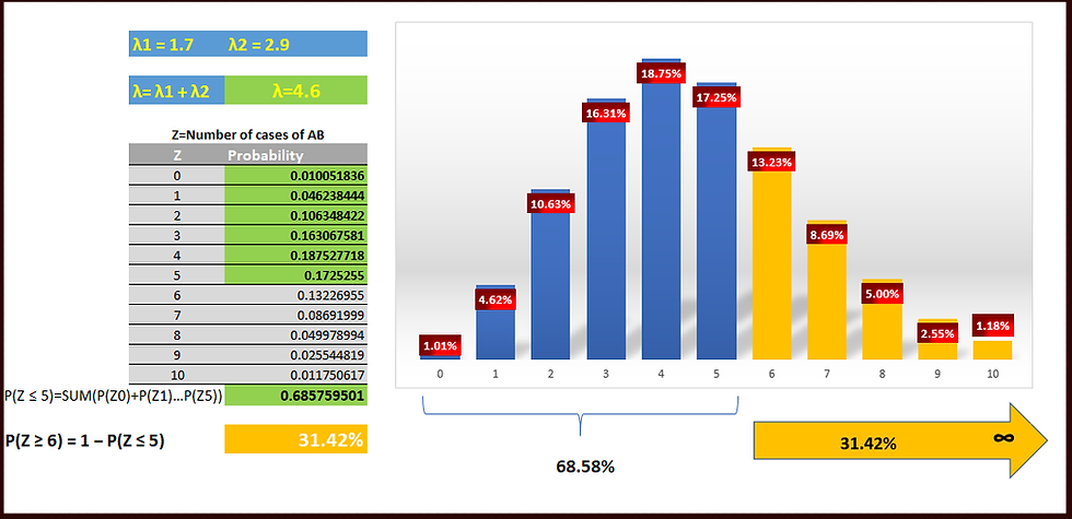
Example: Disease Incidence. [Sum of two Poisson variables]
Suppose that:
disease A occurs with incidence 1.7 per million
disease B occurs with incidence 2.9 per million.
Statistics are compiled, in which these diseases are not distinguished, but simply are all called cases of disease “AB”.
What is the probability that a city of 1 million people has at least 6 cases of AB?
Fitting a Poisson distribution (1.1)
Consider the two sequences of birth times we saw at the beginning. Both of these examples consisted of a total of 44 births in 24 hour intervals. Therefore the mean birth rate for both sequences is 44 / 24 = 1.8333.
What would be the expected counts if birth times were really random i.e. what is the expected histogram for a Poisson random variable with mean rate λ = 1.8333? Using the Poisson formula we can calculate the probabilities of obtaining each possible value.

Fitting a Poisson distribution (1.2)
This consists of 3 steps:
Estimating the parameters of the distribution from the data
Calculating the probability distribution
Multiplying the probability distribution by the number of observations
Using the Poisson to approximate the Binomial
In general,
If n is large (say > 50) and p is small (say < 0.1) then a
Bin(n, p) can be approximated with a Po(λ) where λ = np
Why would we use an approximate distribution when we actually know the exact distribution?
The exact distribution may be hard to work with.
The exact distribution may have too much detail. By using the approximate distribution, we focus attention on the things we’re really concerned with.
Examples: Drownings in Egypt.
The data are given as counts of the number of months in which a given number of drownings occurred.

Do these drowning events occur randomly in time?
Assume these events are independent and occur randomly in time.
Notations:
We imagine there are a large number n of people in the population,
each of whom has an unknown probability p of drowning in any given month.
Then the number of drownings in a month has Bin(n, p) distribution. In order to use this model, we need to know what n and p are. That is, we need to know the size of the population, which we don’t really care about.
The expected (mean) number of monthly drownings is np, and that can be estimated from the observed mean number of drownings. If we approximate the binomial distribution by P o(λ), where λ = np, then we don’t have to worry about the size of the population.
We compute the probabilities for the different possible outcomes assuming the independence assumption < and hence the Poisson model>

The data do not give us strong evidence to reject the neutral assumption, that drownings are independent of one another, and have a constant rate in time.
Example
A life insurance salesman sells on the average 3 life insurance per week. Use Poisson’s law to calculate the probability that in a given [in each] week he will sell some policies.
Some policies = 1 or more.
We can work this out by finding 1 minus the “zero policies” probability.
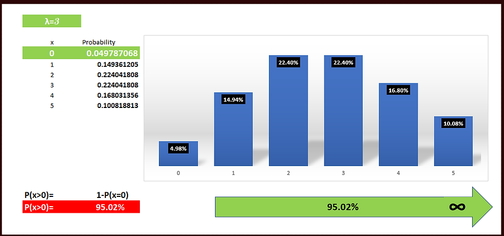
Assuming that there are 5 working days per week, what is the probability that in a given day he will sell 1 policy?
λ=3/5 = 0.6 [ Average number of policies sold per 1 working day.]


Comments